CA - chapter 1 Computer Abstraction and Technology
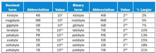
우선 컴퓨터 구조를 시작하기 전에 비트수의 단위에 대한 표를 하나만 보겠다.
공부에 참고한 책은 Computer Oraganization And Design - The HardWare/Software interface, RISC-V Edition(David A. Patterson)으로 뒤에 나올 operand와 같은 내용들을 RISC-V의 기준으로 할 것이다.
◼︎ 컴퓨터 구조 분야의 일곱가지 위대한 아이디어
컴퓨터가 발전하는데에 있어 기여를 크게한 7개의 아이디어에 대해 알아볼 것이다.
- 추상화(Abstraction)
하위 계층의 세부적인 것들이 상위 계층에 보이지 않게 하는 것이다.
ex) low-level language, high level language - 자주 생기는 일을 빠르게(Common case fast)
자주 일어나는 일을 빠르게 하면 성능이 개선된다. - 병렬성(Parallelism)
동시에 작동하면 성능이 개선된다. - 파이프라이닝(Pipelining)
병렬성의 특별한 형태이다. - 예측(Prediction)
예측이 맞으면 빠르게 생략 가능하다. - 메모리 계층구조(Memory heirarchy)
위에 있을수록 빠르지만 용량이 작고 아래로 갈수록 느리지만 용량이 큰 구조 - 여유분을 이용한 신용도 개선(Dependability)
소자가 고장나더라도 대치할 수 있는 여유분이 있으면 신용도가 올라간다 -> Moore’s law
◼︎ 프로세와 메모리 생산 기술
트랜지스터 - 전기로 제어되는 on/off 스위치
집적회로 - 여러개의 트랜지스터를 집적시킨 칩
VSLI - 초대규모집적회로
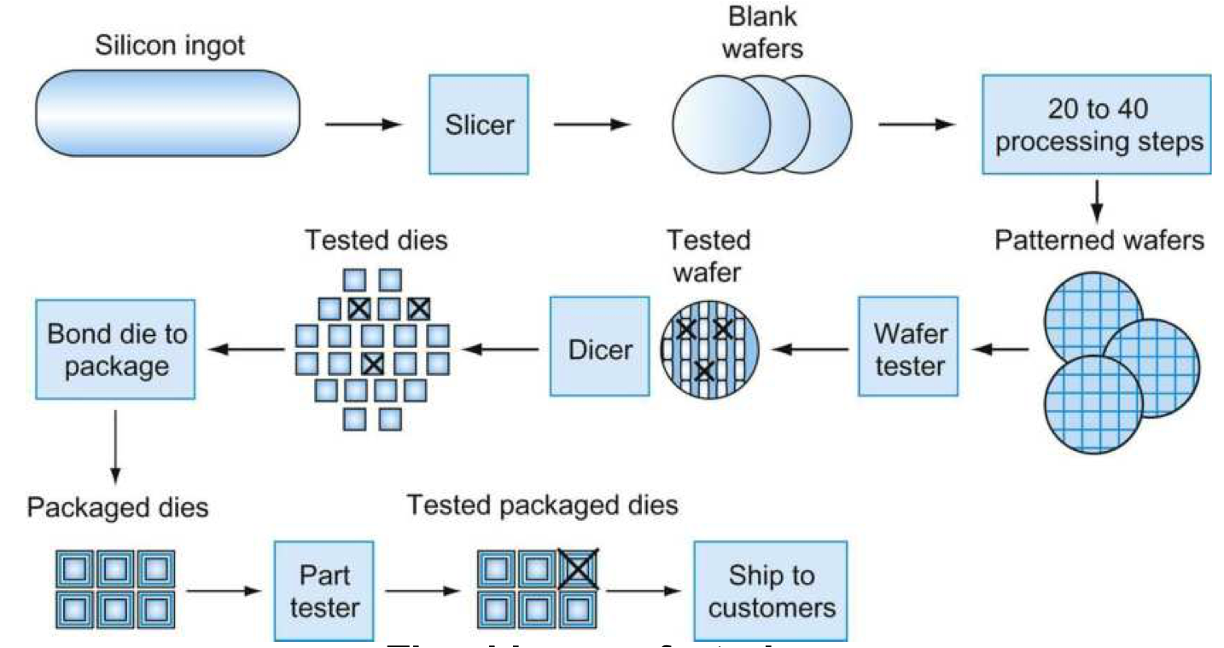
이런 과정을 통해 반도체를 만들게 되는데 이 반도체는 수율과 같은 요소로 판단을 하게 된다.
Cost per die(다이 하나당 가격) = Cost per wafer(웨이퍼당 가격) / {Dies per wafer(웨이퍼 하나에 있는 다이의 개수) X Yield(수율)}
Dies per wafer(웨이퍼 하나에 있는 다이의 개수) = Wafer area(웨이퍼의 면적)/Die area(다이의 면적)
Yield(수율) = 1/(1+ Defects per area(면적에 있는 결함 개수) X Die area/2$)^2$
◼︎ 성능
성능을 판단하는 요소는 굉장히 다양할 수 밖에 없다. 응답시간(Response time)_실행시간(Execution time)이 중요하기도 하고 처리량(Througput)_대역폭(Bandwidth)가 더 중요할 수도 있다. 보통 이 두 가지가 변화면 성능의 변화가 생기게 되는 것이다.
Response time(Execution time)
실행시간을 성능으로 본 식은 다음과 같다.
Performance(성능) = 1 / Execution time(실행시간)
즉, 다음 관계들을 만족하게 된다.
$\mathrm{Perform}_x > \mathrm{Perform}_y$
$\frac{1}{\mathrm{Execution\,time}_x} > \frac{1}{\mathrm{Execution\,time}_y}$
$\mathrm{Execution\,time}_x < \mathrm{Execution\,time}_y$
X is n times faster than Y라고 하면
$\frac{\mathrm{Perform}_x}{\mathrm{Perform}_y} = \frac{\mathrm{Execution\,time}_y}{\mathrm{Execution\,time}_x} = n$
How to measure time
그럼 이 실행시간을 재기 위해서는 어떻게 해야하는 걸까? 우리는 이걸 위해 CPU execution time(CPU time)이란 것을 설정한다. 이것은 user CPU time 과 system CPU time을 합친것이고 CPU의 performance를 뜻하게 된다. User CPU time은 프로그램 자체에 소비된 CPU time이고 system CPU time은 프로그램 실행을 위해 운영체제가 소비한 CPU time인데 이것을 정확히 구분해서 구하는 것은 쉽지 않다. 그래서 경과시간을 기준으로 한다.
CPU clocking
CPU는 항상 clock을 가지게 된다.
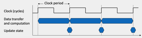
그림과 같이 clock의 한번 주기를 clock period라고 하고 그것의 역수는 clock frequency(rate)라고 한다.
이를 이용해 프로그램에 대한 실행시간을 구할 수 있게 된다.
$\begin{aligned} \mathrm{CPU\,execution\,time\,for\,a\,program(CPU\,time)} & = \mathrm{CPU\,clock\,cycle} \times \mathrm{Clock\,time} \,(N \times t) \newline & = \mathrm{CPU\,clock\,cycle}\, / \,\mathrm{Clock\,rate} \,(N \times f) \end{aligned}$
그러면 여기서 사용한 $\mathrm{CPU\,clock\,cycle}$은 어떻게 구하는 것일까? 이 식은 다음과 같다.
$\mathrm{CPU\,clock\,cycle} = \mathrm{Instruction\,for\,a\,program}(명령어 \, 수) \times \mathrm{Average\,clock\,cycles\,per\,instruction}(CPI)$
우리는 $\mathrm{Average\,clock\,cycles\,per\,instruction}$을 줄여서 CPI라고 부를 것이다.
최종적으로 CPU time에 대한 공식은 다음과 같다.
$\begin{aligned} \mathrm{CPU\,execution\,time\,for\,a\,program(CPU\,time)} & = \mathrm{Instruction\,for\,a\,program} \times \mathrm{Average\,clock\,cycles\,per\,instruction} \times \mathrm{Clock\,time} \,(N \times t) \newline &= \mathrm{Instruction\,for\,a\,program} \times \mathrm{Average\,clock\,cycles\,per\,instruction}\, / \,\mathrm{Clock\,rate} \,(N \times f) \end{aligned} $
이것이 CPU의 성능이라고 생각할 수 있다.
만약 cycle에 대한 instruction의 개수가 달라지면 따로따로 생각을 해줘야 한다.
$\mathrm{Clock \, Cycles} = \sum^{n}_{i=1}(\mathrm{CPI_i} \times \mathrm{Instruction \, Count_i})$
이렇게 되면 CPI의 평균값을 구해야 한다.
$\begin{aligned} \mathrm{CPI} &= \frac{\mathrm{Clock \, Cycles}}{\mathrm{Instruction \, Count}} \newline &= \sum^{n}_{i=1}(\mathrm{CPI_i} \times \frac{\mathrm{Instruction \, Count_i}}{\mathrm{Instruction \, Count}}) \end{aligned} $
The Big Picture(Iron law)
$\mathrm{CPU \, Time} = \frac{\mathrm{Instruction}}{\mathrm{Program}} \times \frac{\mathrm{Clock \, cycles}}{\mathrm{Instruction}} \times \frac{\mathrm{Seconds}}{\mathrm{Clock \, cycles}}$
◼︎ 전력 장벽
Power = Capacitive load $\times$ $\mathrm{Voltage}^2 \times$ Frequency